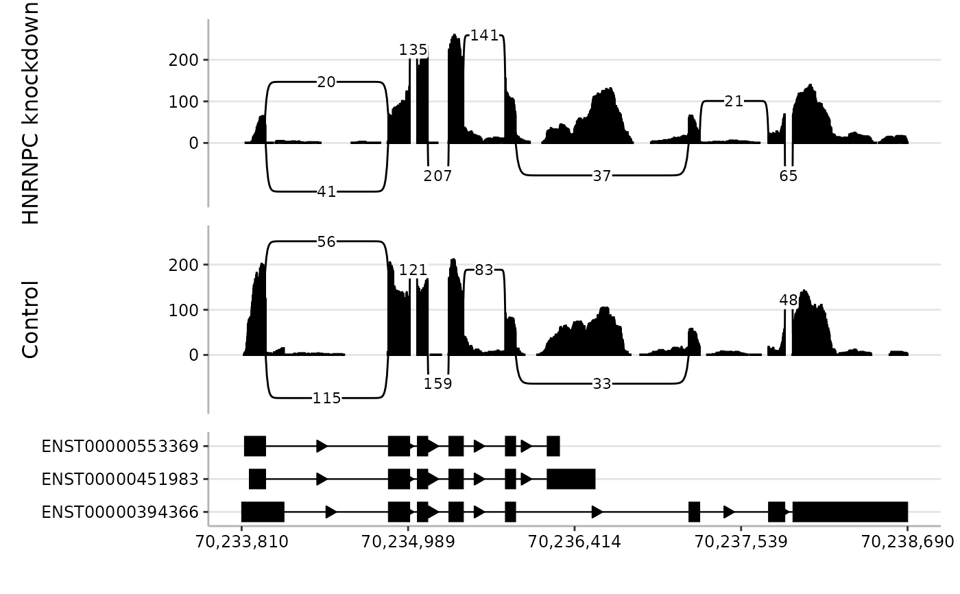
Visualise RNA-seq alignments as sashimi-style plots

spliceTerrain() draws sashimi-style plots for one or more BAM files over a genomic region. Plots combine per-base fragment coverage, splice junction arcs, optional transcript annotation, and highlighted regions. Intronic or otherwise uninformative gaps can be compacted so the plotting area is focused on observed or annotated features.

Usage

spliceTerrain(
  bam,
  region,
  annotation = NULL,
  junction_usage = NULL,
  junction_usage_label_sep = "\n",
  highlight = NULL,
  strandedness = "unstranded",
  min_mapq = 0,
  min_coverage = 0,
  min_junction_reads = 10,
  lib_size = NULL,
  norm_factors = NULL,
  normalise_to = NULL,
  compress_introns = TRUE,
  intron_width = 50,
  min_arrow = intron_width + 1,
  common_y = FALSE,
  arc_height = 1,
  arc_side = c("both", "above", "below"),
  arc_scale = FALSE,
  colours = "black",
  highlight_colour = scales::alpha("red", 0.2),
  anno_fill_by = NULL,
  anno_fill_colours = NULL,
  anno_label_by = NULL,
  anno_label_colour = "white",
  anno_label_size = 3,
  junc_text_size = 3,
  panel_heights = 1,
  axis_title_size = 12,
  axis_text_size = 9,
  return_ctx = FALSE,
  ctx = NULL,
  annotated_junctions = FALSE
)

Arguments

bam: Character vector of BAM file paths. If unnamed, sample labels are derived from BAM basenames with the .bam suffix removed. If names are supplied, all names must be non-empty and unique. BAM files must be indexed for region-restricted import. Index files should be discoverable by Rsamtools using standard same-directory naming, such as file.bam.bai. Single-end and paired-end BAMs are both supported; paired-end status is detected from the BAM flags. For paired-end BAMs, mapped reads are retained even when their mates are unmapped.
region: Genomic interval to plot. May be a GRanges, a GRangesList, or a character string coercible to GRanges, such as "chr:start-end" or "chr:start-end:strand". Commas, spaces, and en/em dashes in character regions are normalised before coercion. If multiple ranges are supplied, they must all be on the same seqname and are reduced to a single span used as the BAM query and plotting window. Supplied Seqinfo metadata is preserved. Use consistent genome assembly identifiers and sequence lengths for the region, annotation, and overlays; known metadata conflicts are rejected by the overlap operations.
annotation: Optional annotation track. Must be a GRangesList, with each list element representing one feature group such as a transcript model. Each group is drawn on its own annotation row. List element names are used as y-axis labels; if absent, default group labels are generated. Supplied names must be non-empty and unique. Annotation groups are retained in full when they overlap the plotting region and are clipped to the plotting window when drawn. All ranges in a retained group must be on the plotting seqname and share one strand.
junction_usage: Optional genomic interval(s) selecting junctions for local usage percentages. Accepts the same formats as region. Junctions with either anchor overlapping the interval(s) are selected. Each percentage is that junction's fraction of summed fragment support among all selected, eligible imported junctions in its sample, before display filtering or clipping. A single shared splice site gives the clearest interpretation; a range can combine multiple sites. This is not an event-level percent-spliced-in estimate. Anchors are the first and last intronic bases.
junction_usage_label_sep: Character scalar inserted between junction counts and percentages when junction_usage is supplied. Defaults to "\n"; use " " to keep percentages inline with counts.
highlight: Optional interval(s) to highlight. Accepts the same formats as region. Multiple ranges may be supplied. Highlighted intervals are drawn as shaded vertical bands spanning the full panel height. Only the portion overlapping the plotting window is drawn. Returned contexts keep the full retained genomic intervals in highlight.
strandedness: Library strandedness for each BAM. Must be one of "unstranded", "forward", or "reverse", and may be supplied either as a single value applied to all BAMs or as one value per BAM. Use "unstranded" when reads from both strands should be included. For stranded paired-end BAMs, this value is passed to readGAlignmentsList as strandMode, which uses the read-one/read-two flags for both complete pairs and singletons. If region includes a strand and strandedness is not "unstranded", imported alignments are restricted to overlaps on the resolved region strand.
min_mapq: Integer scalar. Minimum mapping quality (MAPQ) for alignments to be imported from the BAM file.
min_coverage: Integer or percentage string. Minimum per-base fragment coverage required for positions to be retained for plotting. Percentage strings such as "10%" are relative to the maximum coverage within the plotting region for each BAM. May be supplied as a single value for all BAMs or as one value per BAM. Per-BAM character vectors may combine whole-number counts and percentage strings.
min_junction_reads: Integer or percentage string. Minimum number of fragments supporting a junction for it to be retained for plotting. Both mates supporting the same junction contribute one count. Percentage strings such as "10%" are relative to the most-supported junction within the plotting region for each BAM. May be supplied either as a single value applied to all BAMs or as one value per BAM. Per-BAM character vectors may combine whole-number counts and percentage strings.
lib_size: Optional numeric vector giving full-library sizes in fragment units, one per BAM file, before restriction to the plotting region. A pair or mapped singleton is one fragment; for single-end libraries, each mapped read is one fragment. When supplied, coverage and junction counts are normalised by effective library size before plotting.
norm_factors: Optional numeric vector of normalisation factors, one per BAM file, such as edgeR TMM normalisation factors. Requires lib_size. Effective library sizes are calculated as lib_size * norm_factors.
normalise_to: Optional numeric scalar giving the target library size used for normalisation. If NULL, counts are normalised to the median effective library size.
compress_introns: Logical scalar. If TRUE, compact gaps between observed or annotated genomic blocks so plotting space is focused on regions containing coverage, junctions, annotations, or supplied overlays. If FALSE, plot genomic coordinates directly.
intron_width: Integer scalar. Approximate plot-space width used for compacted gaps when compress_introns = TRUE.
min_arrow: Integer scalar. Minimum annotation intron width required before drawing directional arrows.
common_y: Logical scalar. If TRUE, use a common y-axis range across all sample panels. If FALSE, each sample panel is scaled independently.
arc_height: Numeric scalar multiplying the default junction arc height. arc_height = 1 uses the default height of 0.15 times the coverage scale; larger values produce taller arcs and greater separation between stacked arcs.
arc_side: Character scalar controlling where junction arcs are drawn. Must be one of "both", "above", or "below". The default "both" alternates arcs above and below the coverage track in genomic sort order.
arc_scale: Logical scalar. If TRUE, scale junction arc line width by junction fragment count after filtering. If FALSE, use a constant line width for all junction arcs.
colours: Character vector of colours used for each sample's coverage bars and junction arcs. Must be either length 1, in which case the same colour is used for all BAMs, or the same length as bam, in which case one colour is used per sample.
highlight_colour: Fill and border colour used for highlighted regions. The default is a semi-transparent red produced with scales::alpha("red", 0.2).
anno_fill_by: Optional character scalar naming a metadata column in annotation used to group annotation features for fill colouring. Use "group" to colour by transcript/group. Values in this column are treated as discrete groups, not as continuous values or literal colour names or hex codes.
anno_fill_colours: Optional vector of colours used when anno_fill_by is supplied. Use this argument to set annotation fill colours. If named, names should match values in the selected fill column.
anno_label_by: Optional character scalar naming a metadata column in annotation to display as text within annotation features.
anno_label_colour: Character scalar giving the colour used for annotation labels.
anno_label_size: Numeric scalar giving the text size used for annotation labels.
junc_text_size: Numeric scalar giving the size of junction count labels. Passed to ggplot2::geom_label() for junction annotations.
panel_heights: Numeric vector controlling relative heights of the plot panels. Must be length 1 or the number of BAM sample panels plus one additional value if an annotation panel is shown. When an annotation panel is shown, its height is specified by the final value.
axis_title_size: Numeric scalar giving the axis title text size used in the final plot theme.
axis_text_size: Numeric scalar giving the axis tick-label text size used in the final plot theme.
return_ctx: Logical scalar. If FALSE, return the assembled sashimi plot. If TRUE, return the processed context list after BAM import, coverage and junction summarisation, and filtering, but before coordinate mapping or plot assembly. Coordinate-bearing fields in the returned context use genomic coordinates.
ctx: Optional context list previously returned by spliceTerrain(..., return_ctx = TRUE). When supplied, BAM import, summarisation, and filtering are skipped. Plot-space coordinates are rebuilt from the context's genomic data before drawing the plot. No other arguments may be supplied with ctx; plotting options can instead be modified in the context itself.
annotated_junctions: Logical scalar. If TRUE, junctions that exactly match an intron implied by annotation are drawn with solid arcs and unmatched junctions are drawn with dashed arcs. Matching uses seqname, start, and end coordinates and ignores strand. Requires annotation.

Value

If return_ctx = FALSE, a patchwork object containing one sample panel per BAM file plus an optional annotation panel.

If return_ctx = TRUE, a named list containing validated settings and processed alignment, coverage, junction, annotation, and overlay data. All coordinate-bearing fields use genomic coordinates; plot-space data are generated internally when the context is plotted.

The gal field contains one alignment object per BAM: a GAlignments for single-end input or a GAlignmentsList for paired-end input. Paired-end list elements group the imported mates and include mapped singleton reads.

The cov and juncs fields store fragment summaries. Their coverage_raw columns contain unnormalised fragment counts, while coverage contains the values used for plotting, normalised when lib_size is supplied. The gal field retains the imported alignments rather than collapsed coverage or junction data.

juncs_all stores the unfiltered junction reference. The usage_fraction column in juncs contains fractions on the 0–1 scale; NA denotes an unselected junction or undefined percentage. Fractions are recalculated from juncs_all before each plot is drawn.

In the returned plot, the x-axis is shared across panels. Tick labels are shown in genome coordinates, including when introns are compressed.

Details

The plot is built in three conceptual steps:

Alignments overlapping region are imported from each BAM file. Unmapped, secondary, and supplementary alignments are ignored, and min_mapq is applied during import.
Fragment coverage and splice junction support are summarised from the imported alignments and filtered by min_coverage and min_junction_reads.
If compress_introns = TRUE, a plot-space map is constructed to compact gaps between observed or annotated genomic blocks. Coverage, junctions, annotation, and optional overlays are then mapped into this compacted coordinate system.

For BAMs detected as paired-end, alignments flagged as paired are imported as groups containing complete pairs or mapped singletons. A mapped read does not require a mapped mate to contribute to the plot. Each imported group is treated as one fragment. For single-end input, each read is one fragment. Coverage uses the union of each fragment's aligned blocks. Overlapping mates contribute at most one count per position. Introns and unsequenced gaps between mates are not filled. Each fragment contributes at most one count per distinct junction, even when both mates cross it; a fragment can support multiple different junctions. Independent fragments are counted separately, including those with identical coordinates. This is not PCR/UMI deduplication. Retaining singletons avoids losing their signal when mate-mapping success differs between samples.

region, junction_usage, and highlight may be supplied as genomic ranges or as strings coercible to GRanges. If multiple ranges are supplied for region, they must all be on the same seqname; their span is used as the BAM query and plotting window. Optional genomic overlays are retained when they overlap the plotting region and are clipped to the plotting window when drawn.

junction_usage and highlight are optional selections:

junction_usage selects junctions by their intronic anchors. Percentages use raw fragment support after import/MAPQ/strand filtering, before min_junction_reads filtering and plotting-window exclusion. Hidden junctions remain in the denominator, so visible percentages need not sum to 100. A junction is counted once in the denominator even when both anchors or multiple selection intervals match it. Different junctions from one fragment each contribute their support; these are junction fractions, not fractions of unique molecules across the whole selection.
highlight marks one or more genomic intervals to draw attention to a subregion, such as an exon, splice site, or event.

Usage percentages are computed separately for each sample and are unchanged by library-size normalisation or coordinate compression. Labels are rounded to one decimal place. If no selected junction has positive support, no usage percentage is shown. The denominator is conditional on the imported data: changing the BAM query region, MAPQ threshold, or strand selection can change which evidence is available.

The arguments strandedness, min_coverage, min_junction_reads, and colours may each be supplied either as length 1, in which case the value is recycled across all BAMs, or as one value per BAM.

When lib_size is supplied, coverage and junction counts are normalised to a common effective library size before plotting. Effective library sizes are calculated as lib_size * norm_factors, with norm_factors = 1 when not supplied. If normalise_to = NULL, counts are normalised to the median effective library size. Filtering thresholds min_coverage and min_junction_reads are always applied to raw counts before normalisation. Percentage thresholds are calculated separately for each BAM from the maximum raw value within the plotting region.

Strand filtering is applied after BAM import. Unstranded libraries retain alignments from both strands. For stranded libraries, reads are interpreted according to strandedness; when the resolved region has a specific strand, alignments are then restricted to that strand.

When compress_introns = TRUE, the plot uses compacted coordinates internally, but x-axis tick labels are reported as approximate genomic coordinates.

Annotation is drawn on a separate panel beneath the sample panels. Highlighted intervals are overlaid across both sample and annotation panels when present.

For advanced workflows, return_ctx = TRUE can be used to inspect or modify processed genomic data before plotting. The returned context is a named list containing genomic summaries and plotting settings. Fields such as cov, juncs, juncs_all, annotation, junction_usage, and highlight all use genomic coordinates. Passing the modified context through ctx rebuilds the coordinate map and redraws the plot without reading the BAM files again.

Coverage and junctions in a returned context have already been summarised, filtered, and normalised. Changing processing settings such as min_mapq, min_coverage, min_junction_reads, or lib_size does not repeat those processing steps; modify ctx$cov or ctx$juncs directly instead. Plotting settings such as colours, arc_side, and compress_introns may be changed in the context before replotting.

juncs_all retains the eligible junction summaries on the plotting chromosome before display filtering or clipping, including junctions outside the plotting window. It is the reference for usage calculations when a context is replotted. Filtering ctx$juncs changes only the display; modify ctx$juncs_all if you intend to change the usage reference. The reference must retain one row per sample/junction and its non-negative coverage_raw counts. Changing ctx$junction_usage to another GRanges selection recalculates percentages from this reference. The replacement selection must overlap the plotting region and have compatible genomic metadata.

References

Katz Y et al. (2015). Quantitative visualization of alternative exon expression from RNA-seq data. Bioinformatics, 31(14), 2400–2402. doi:10.1093/bioinformatics/btv034 .

Robinson MD and Oshlack A (2010). A scaling normalization method for differential expression analysis of RNA-seq data. Genome Biology, 11, R25. doi:10.1186/gb-2010-11-3-r25 .

Zarnack K et al. (2013). Direct Competition between hnRNP C and U2AF65 Protects the Transcriptome from the Exonization of Alu Elements. Cell, 152(3), 453–466. doi:10.1016/j.cell.2012.12.023 .

Examples

if (
  requireNamespace("RNAseqData.HNRNPC.bam.chr14", quietly = TRUE) &&
  requireNamespace("EnsDb.Hsapiens.v75", quietly = TRUE) &&
  requireNamespace("AnnotationFilter", quietly = TRUE) &&
  requireNamespace("ensembldb", quietly = TRUE)
) {
  bams <- RNAseqData.HNRNPC.bam.chr14::RNAseqData.HNRNPC.bam.chr14_BAMFILES
  bams <- bams[c(7, 1)]
  names(bams) <- c("HNRNPC knockdown", "Control")
  region <- "chr14:70,233,810-70,238,690"

  annotation <- ensembldb::exonsBy(
    EnsDb.Hsapiens.v75::EnsDb.Hsapiens.v75,
    by = "tx",
    filter = AnnotationFilter::GeneIdFilter("ENSG00000100650")
  )
  annotation <- annotation[1:3]
  ensembldb::seqlevelsStyle(annotation) <- "ucsc"

  spliceTerrain(bam = bams, region = region)

  spliceTerrain(
    bam = bams,
    region = region,
    lib_size = c(40e6, 55e6),
    norm_factors = c(0.95, 1.08),
    common_y = TRUE
  )

  spliceTerrain(
    bam = bams,
    region = region,
    annotation = annotation,
    anno_fill_by = "group",
    anno_fill_colours = c(
        ENST00000553369 = "#66C2A5",
        ENST00000394366 = "#8DA0CB",
        ENST00000451983 = "#FC8D62"
    ),
    anno_label_by = "exon_rank",
    anno_label_colour = "black",
    junction_usage = "chr14:70234854-70234854",
    highlight = "chr14:70233810-70234097",
    arc_height = 2,
    arc_side = "above",
    arc_scale = TRUE,
    common_y = TRUE,
    colours = c("darkblue", "darkred"),
    highlight_colour = scales::alpha("gold", 0.25),
    anno_label_size = 2,
    panel_heights = c(2, 2, 1)
  )

  ctx <- spliceTerrain(
    bam = bams,
    region = region,
    annotation = annotation,
    min_junction_reads = 1,
    panel_heights = c(2, 2, 1),
    return_ctx = TRUE
  )
  ctx$juncs <- ctx$juncs[ctx$juncs$coverage >= 20]
  spliceTerrain(ctx = ctx)
}