Creating Sashimi-Style Plots with `spliceTerrain`

Installation and setup

BiocManager is recommended for installing the packages required in this vignette. BiocManager handles installation from Bioconductor, CRAN and GitHub repositories.

if (!"BiocManager" %in% rownames(installed.packages()))
    install.packages("BiocManager")
pkgs <- c(
    "spliceTerrain", "RNAseqData.HNRNPC.bam.chr14", "EnsDb.Hsapiens.v75",
    "AnnotationFilter", "ensembldb", "GenomicRanges", "scales", "pander",
    "GenomeInfoDb"
)
BiocManager::install(pkgs, update = FALSE)

library(spliceTerrain)
library(RNAseqData.HNRNPC.bam.chr14)
library(EnsDb.Hsapiens.v75)
library(AnnotationFilter)
library(ensembldb)
library(GenomicRanges)
library(scales)
library(pander)
library(GenomeInfoDb)

Quick start

At a minimum, spliceTerrain() needs BAM file paths and a genomic interval. Here we use BAM files from RNAseqData.HNRNPC.bam.chr14, selecting one HNRNPC knockdown sample and one control sample from the study by Zarnack et al. (Zarnack et al. 2013) (ArrayExpress accession E-MTAB-1147). The region can be supplied as a single character string.

bams <- RNAseqData.HNRNPC.bam.chr14_BAMFILES[c(7, 1)]
region <- "chr14:70,233,810-70,238,690"

spliceTerrain(bam = bams, region = region)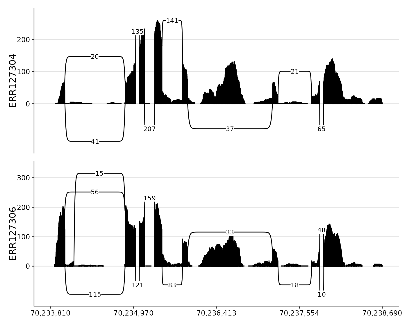

Introduction

Sashimi plots visualise RNA-seq alignments across a genomic interval. They combine coverage tracks with arcs representing splice junction support (Katz et al. 2015). spliceTerrain reports both coverage and junction support in fragment-level units. This makes them useful for inspecting transcript structure, exon usage, alternative splice sites, intron retention, and differences in junction usage between samples.

Motivation

spliceTerrain was designed to fit into R/Bioconductor workflows. Candidate regions, exon models, and features of interest are often already represented as GRanges or GRangesList objects from GenomicRanges (Lawrence et al. 2013). spliceTerrain allows reuse of these objects for regions, transcript annotation, and highlights alongside indexed BAM files, within the same R session. For example, exon models retrieved from an EnsDb object can become annotation rows without first exporting them to an annotation file.

spliceTerrain brings these inputs together in a focused, sample-resolved sashimi workflow. It returns a patchwork plot or an inspectable genomic context. Its genomic summaries and plotting settings can be edited and replotted.

spliceTerrain displays one panel per BAM for visual inspection of local splicing patterns. It does not perform differential-splicing testing, estimate event-level PSI, or infer transcript isoforms.

Several established tools support related visualisation tasks:

Gviz provides genomic tracks, including BAM-backed coverage and sashimi plots (Hahne and Ivanek 2016).
ggbio provides genomic visualisation based on ggplot2, with support for Bioconductor objects and transcript-based splice summaries (Yin et al. 2012).
SpliceWiz provides coverage and sashimi plots within an alternative-splicing analysis workflow. Its event-normalised coverage plots offer an alternative view of splicing differences, summarising replicates by condition rather than relying on individual-sample sashimi plots (Wong et al. 2024).
ggsashimi provides a command-line sashimi plotting workflow with sample overlays and aggregation (Garrido-Martín et al. 2018).

spliceTerrain focuses on sample-resolved sashimi plots within R/Bioconductor workflows. It is particularly useful when regions and annotations are already represented as genomic objects and plots need iterative refinement. It combines:

Editable genomic summaries: inspect or modify coverage, junctions, and settings in a returned context, then replot without importing the BAM files again.
Coverage-aware compression: preserve selected blocks defined by coverage, annotation, and junction anchors while shortening gaps. Coverage retained after filtering can preserve regions within annotated introns at their original width.
Fragment-level support: count overlapping mates once per covered base and once per distinct junction, while retaining mapped singletons.
Stable local junction fractions: calculate usage against the pre-display junction reference, so hiding arcs does not change the remaining percentages.
Integrated sample normalisation: apply supplied library sizes and optional normalisation factors consistently to coverage and junction support, while retaining raw fragment counts for filtering.

These choices offer specific contrasts with existing workflows. When compression is enabled, ggsashimi uses junction-derived, length-dependent shrinking, whereas spliceTerrain also uses retained coverage and annotation to define preserved blocks. By default, Gviz and ggsashimi count support at the read level, so both mates can contribute to coverage and junction counts. In contrast, spliceTerrain uses fragment-level counts. spliceTerrain displays transcript annotation alongside observed junction support without assigning that support to transcript models. This complements the transcript-model-based summaries provided by ggbio’s plotSpliceSum().

spliceTerrain exposes sample normalisation through dedicated arguments. Gviz supports custom transformations that can implement similar scaling, whereas the ggsashimi command-line interface has no equivalent library-size normalisation option.

Versions compared: Gviz 1.57.4, ggbio 1.61.0, SpliceWiz 1.15.0, and ggsashimi 1.1.5.

Complete guide

The following sections build up aspects of a more complete plot and introduce the main options available in spliceTerrain(). The examples continue to use the HNRNPC chr14 BAM files from the quick start.

Input BAM files and regions

The bam argument is a character vector of indexed BAM file paths. If the vector is named, those names are used as sample labels in the plot. If it is unnamed, labels are derived from the BAM file names. BAM files must be indexed for region-restricted import. Index files should be discoverable by Rsamtools using standard same-directory naming, typically file.bam.bai.

bams <- RNAseqData.HNRNPC.bam.chr14_BAMFILES[c(7, 1)]
names(bams) <- c("HNRNPC knockdown", "Control")

The region argument can be a character string, a GRanges, or a GRangesList. Character regions may use comma-separated coordinates, such as "chr14:70,233,810-70,238,690". For Bioconductor workflows, using a GRanges object is often more convenient.

Because the example BAM files use UCSC style chromosome names, we also convert the region to UCSC style before plotting.

ensDb <- EnsDb.Hsapiens.v75
region <- transcripts(ensDb, filter = TxIdFilter("ENST00000394366"))
seqlevelsStyle(region) <- "UCSC"
region
#> GRanges object with 1 range and 6 metadata columns:
#>                   seqnames            ranges strand |           tx_id     tx_biotype tx_cds_seq_start tx_cds_seq_end         gene_id         tx_name
#>                      <Rle>         <IRanges>  <Rle> |     <character>    <character>        <integer>      <integer>     <character>     <character>
#>   ENST00000394366    chr14 70233810-70238690      + | ENST00000394366 protein_coding         70234874       70238178 ENSG00000100650 ENST00000394366
#>   -------
#>   seqinfo: 1 sequence from hg19 genome

If multiple ranges are supplied, spliceTerrain() reduces them to a single span on one chromosome and uses that span as the BAM query and plotting window. The span is the smallest continuous interval containing all supplied ranges: it starts at the lowest start coordinate and ends at the highest end coordinate.

Adding transcript annotation

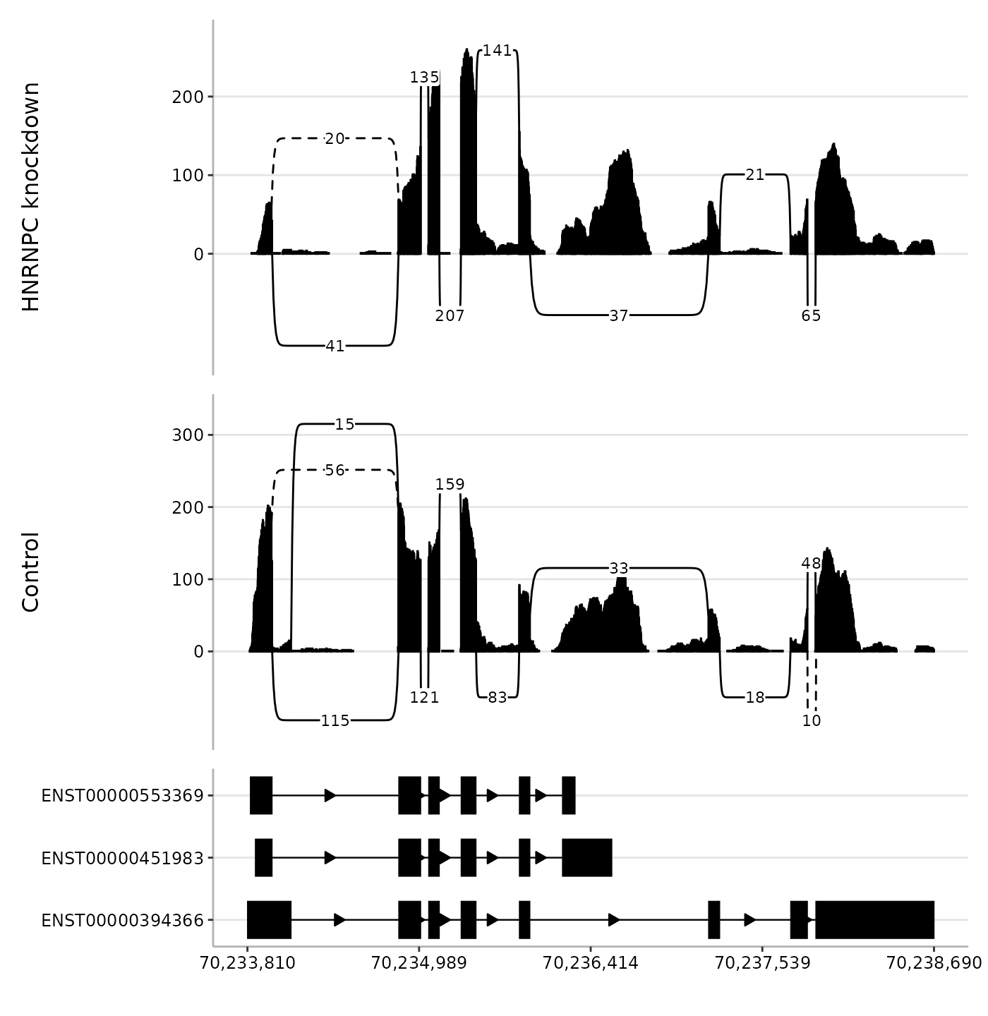
Transcript models can be displayed with the annotation argument. This must be a GRangesList, where each list element represents one transcript or feature group. The names of the list elements are used as y-axis labels in the annotation panel. When annotation is present, the final plot contains one panel per BAM file plus one annotation panel. The relative heights of these panels are controlled with panel_heights, where the final value corresponds to the annotation panel. Setting annotated_junctions = TRUE distinguishes junctions that exactly match an intron in the supplied annotation with solid arcs, while unmatched junctions are drawn with dashed arcs. Junction classification is relative to the supplied annotation, so known junctions may appear unmatched when only a subset of transcripts is provided.

For this vignette, the plotting region covers the SRSF5 gene. We retrieve exon ranges for the gene and keep a small number of transcripts so the annotation panel remains readable.

annotation <- exonsBy(
    ensDb, by = "tx", filter = GeneIdFilter("ENSG00000100650")
)
annotation <- annotation[1:3]
seqlevelsStyle(annotation) <- "UCSC"

spliceTerrain(
    bam = bams,
    region = region,
    annotation = annotation,
    annotated_junctions = TRUE,
    panel_heights = c(2, 2, 1)
)

Styling annotation tracks

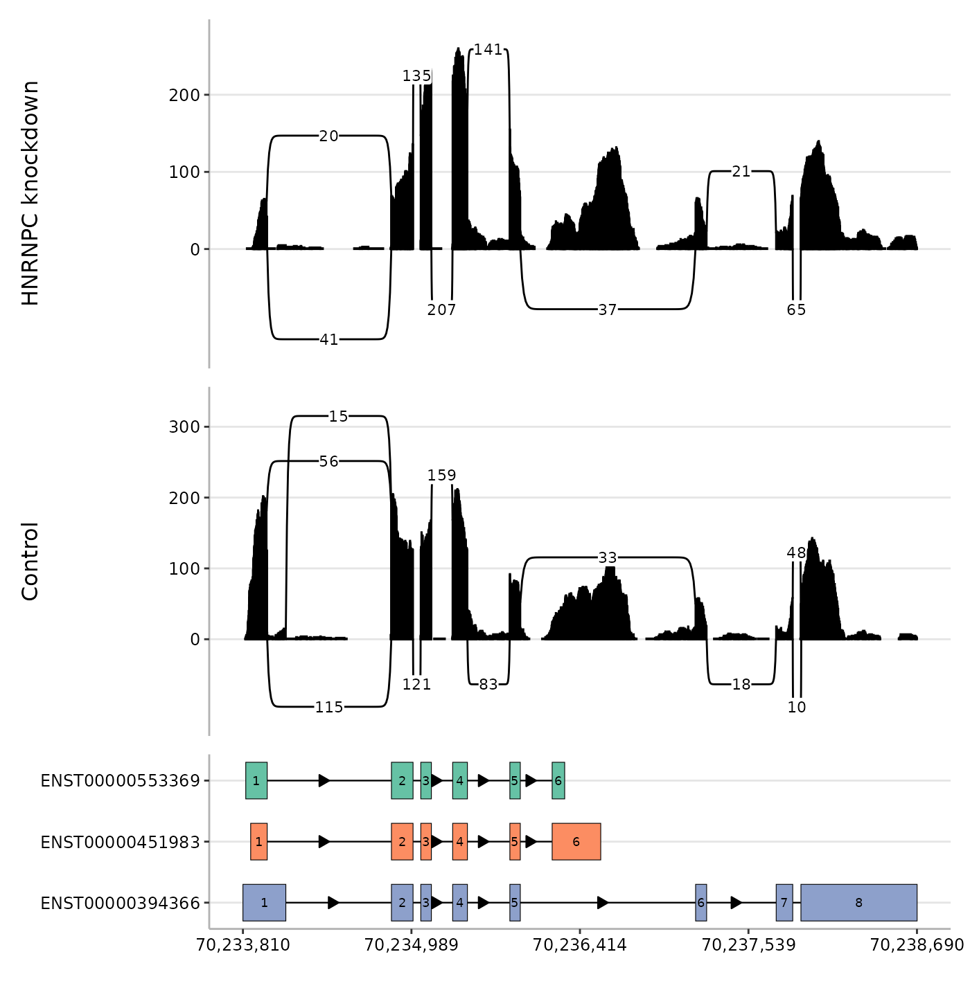
Annotation features can be coloured by a metadata column with anno_fill_by. Use "group" to colour each transcript or feature group separately. Specific fill colours can be supplied with anno_fill_colours.

Text labels can be drawn inside annotation features with anno_label_by. The label colour and size are controlled by anno_label_colour and anno_label_size. The min_arrow argument controls how wide an annotation intron must be before directional arrows are drawn.

spliceTerrain(
    bam = bams,
    region = region,
    annotation = annotation,
    panel_heights = c(2, 2, 1),
    anno_fill_by = "group",
    anno_fill_colours = c(
        ENST00000553369 = "#66C2A5",
        ENST00000394366 = "#8DA0CB",
        ENST00000451983 = "#FC8D62"
    ),
    anno_label_by = "exon_rank",
    anno_label_colour = "black",
    anno_label_size = 2.5,
    min_arrow = 100
)

Highlighting regions of interest

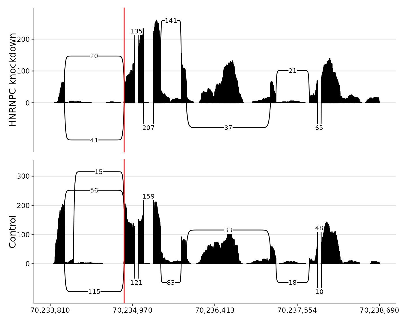
The highlight argument marks one or more genomic intervals with shaded vertical bands. This is useful for drawing attention to a splice site, variant position, alternative exon, or other feature of interest. The highlighted interval can be supplied as a character string or as a GRanges object.

spliceTerrain(
    bam = bams,
    region = region,
    highlight = "chr14:70234854-70234854",
    highlight_colour = "red"
)

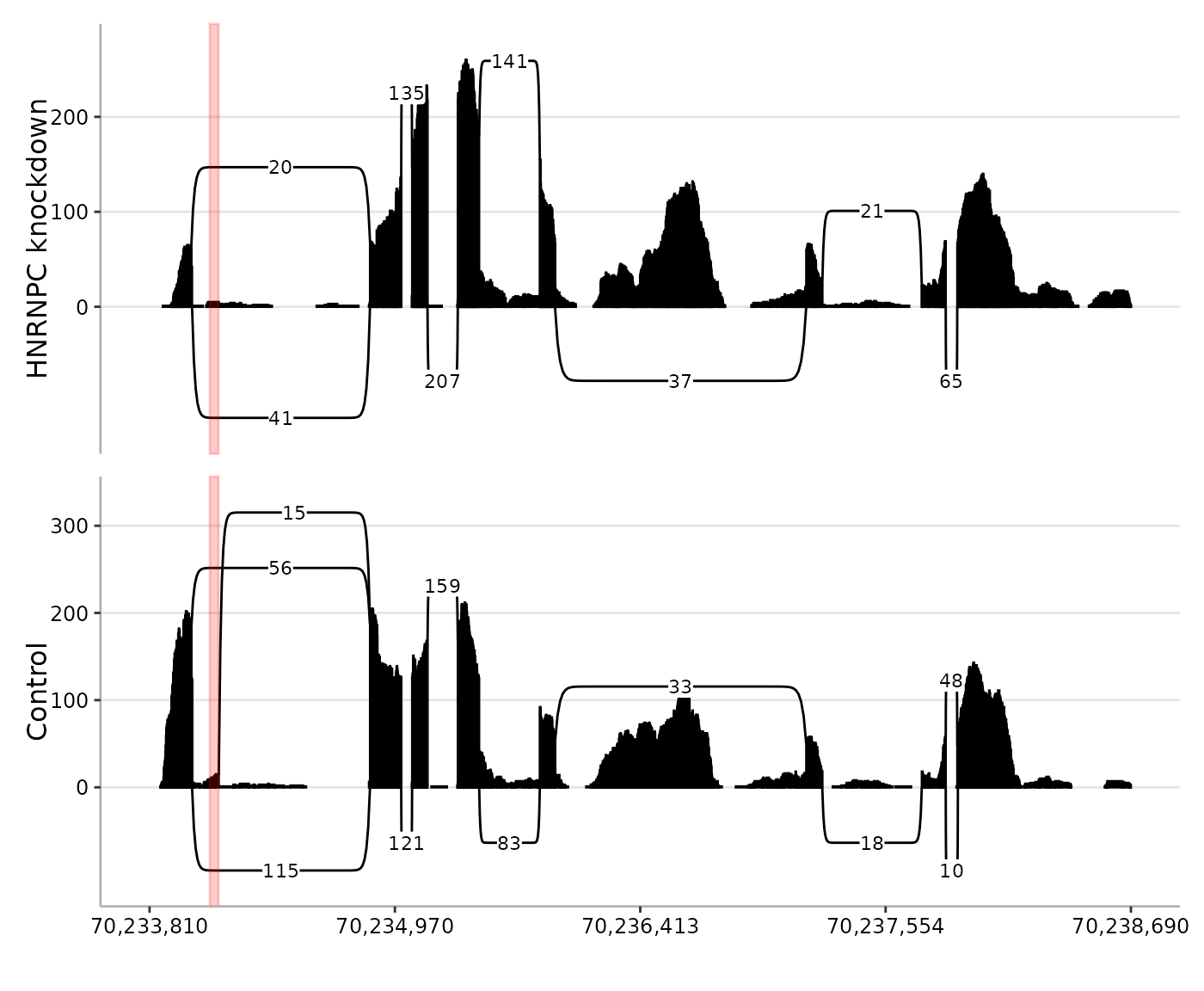
A wider interval can be highlighted with a semi-transparent colour.

spliceTerrain(
    bam = bams,
    region = region,
    highlight = "chr14:70234056-70234097",
    highlight_colour = scales::alpha("red", 0.2)
)

Local junction-usage labels

The junction_usage argument selects junctions by a genomic position or range and labels their relative fragment support within each sample. Junctions are selected when either their start or end anchor overlaps the supplied interval(s). Junction anchors use intronic coordinates: the start anchor is the first base of the intron, and the end anchor is the last base of the intron, not the adjacent exonic bases.

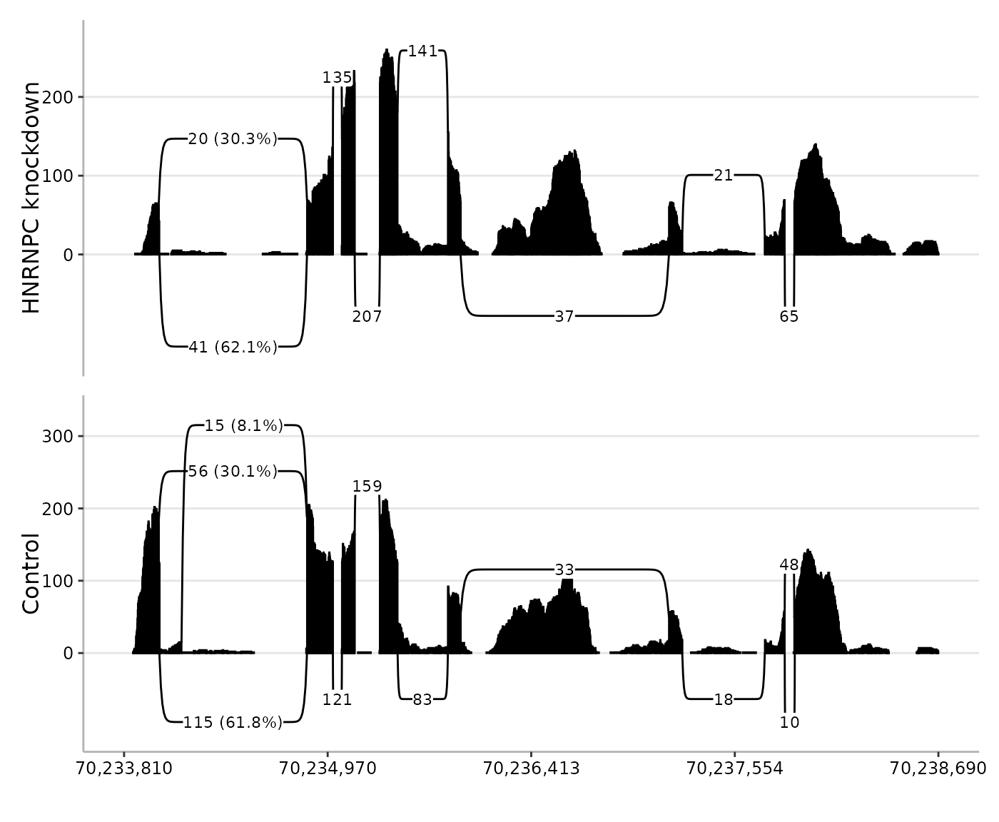
Selecting a single shared splice site gives the cleanest interpretation. For junctions sharing a donor or acceptor, the labels describe their relative support at that site. By default, the junction count and usage percentage are separated by a new line. Use junction_usage_label_sep = " " to display them together on one line.

spliceTerrain(
    bam = bams,
    region = region,
    junction_usage = "chr14:70234854-70234854",
    junction_usage_label_sep = " "
)

A range can also be supplied, including one covering multiple splice sites. It defines a combined set of selected junctions; each junction enters the denominator once, even if both anchors or overlapping intervals select it.

spliceTerrain(
    bam = bams,
    region = region,
    junction_usage = "chr14:70234098-70234854"
)

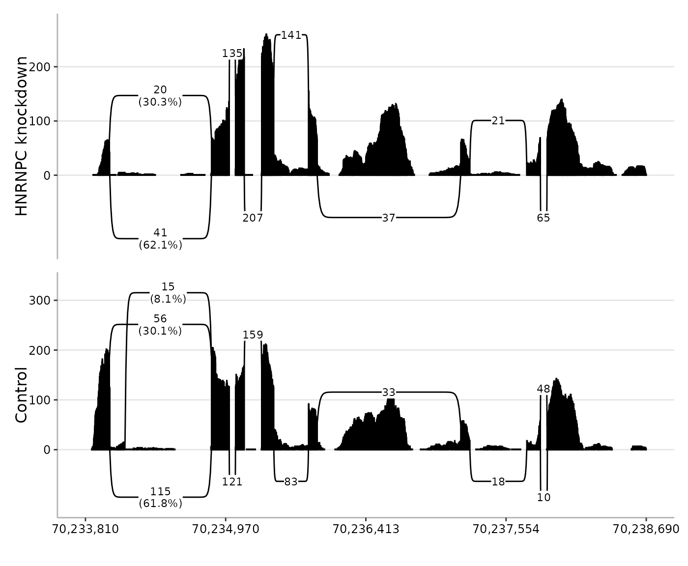
For each sample, the percentage is the junction’s raw fragment support divided by the summed support of all selected, eligible imported junctions. This is calculated after import, MAPQ, and strand filtering, but before min_junction_reads filtering or plotting-window exclusion. An alternative junction remains in the denominator when its arc is hidden. For example, supports of 90 and 9 give 90.9% and 9.1%; hiding the second arc with a threshold of 10 leaves the first label at 90.9%, not 100%. Visible percentages therefore need not sum to 100%. Library-size normalisation does not change the fractions. The reference is conditional on the imported data: changing the query region, MAPQ threshold, or strand selection can change the available evidence.

Why this is not event-level PSI

Consider a cassette exon between an upstream and a downstream exon. In a simplified example, 50 inclusion fragments support both inclusion junctions, and 50 skipping fragments support the direct skipping junction. A range selecting all three junctions gives the following junction-usage labels:

cassette <- data.frame(
    Junction = c("Upstream inclusion", "Downstream inclusion", "Skipping"),
    Fragments = c(50L, 50L, 50L)
)
cassette[["Junction usage (%)"]] <- round(
    100 * cassette$Fragments / sum(cassette$Fragments), 1
)
pander(cassette)

Junction	Fragments	Junction usage (%)
Upstream inclusion	50	33.3
Downstream inclusion	50	33.3
Skipping	50	33.3

The denominator is 150 units of junction support, so each label is 33.3%. There are only 100 fragments in this constructed example, with a known exon inclusion fraction of 50%: each inclusion fragment supports two junctions. Thus the 33.3% labels are not estimates of the cassette exon’s inclusion. Selecting one shared donor or acceptor instead compares one inclusion junction with the skipping junction and gives 50% for each in this example. Ranges remain useful for inspecting broader patterns, but their combined junction fractions should not be interpreted as general event-level percent spliced in (PSI) or transcript-isoform proportions.

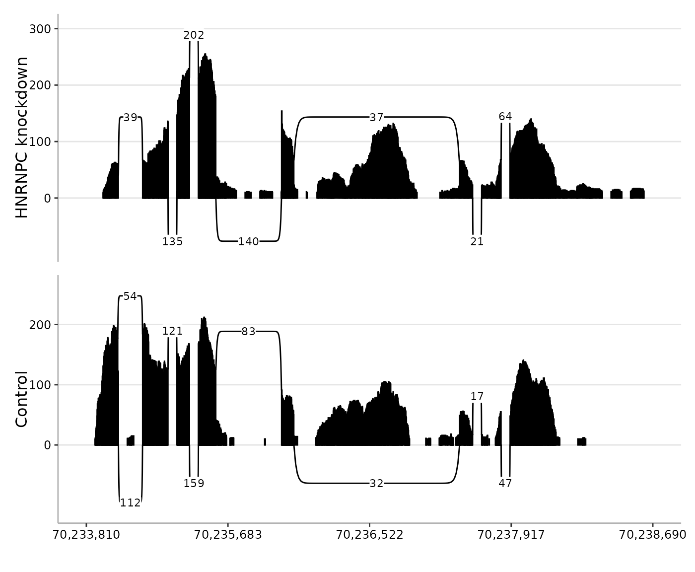
Filtering signal

Three arguments control how much signal is imported and displayed. min_mapq filters alignments by mapping quality during BAM import. min_coverage filters positions by per-base fragment coverage before plotting. min_junction_reads sets the minimum fragment support required to display a junction arc. Both mates supporting the same junction contribute one count. Both thresholds are applied to raw fragment counts before library-size normalisation. The latter two arguments also accept percentage strings such as "10%". Percentage thresholds are calculated separately for each BAM relative to its maximum raw coverage or junction count within the plotting region. When supplying one threshold per BAM, whole-number counts and percentages can be mixed in a character vector.

spliceTerrain(
    bam = bams,
    region = region,
    min_mapq = 10,
    min_coverage = 10,
    min_junction_reads = "10%"
)

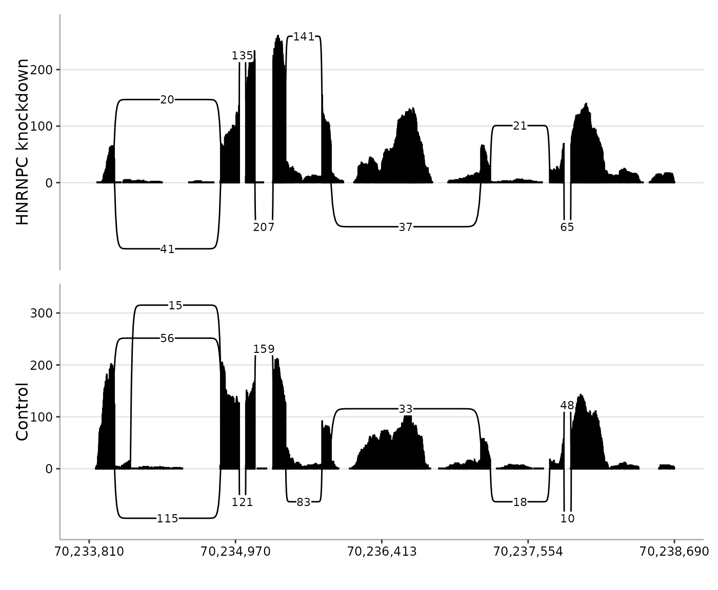
Stranded RNA-seq data

The strandedness argument describes how read strand should be interpreted. It can be one of "unstranded", "forward", or "reverse", and can be supplied either as a single value for all BAM files or one value per BAM file. The example BAM files are unstranded, so both read orientations contain signal from the transcript.

spliceTerrain(
    bam = bams,
    region = region,
    strandedness = "unstranded"
)

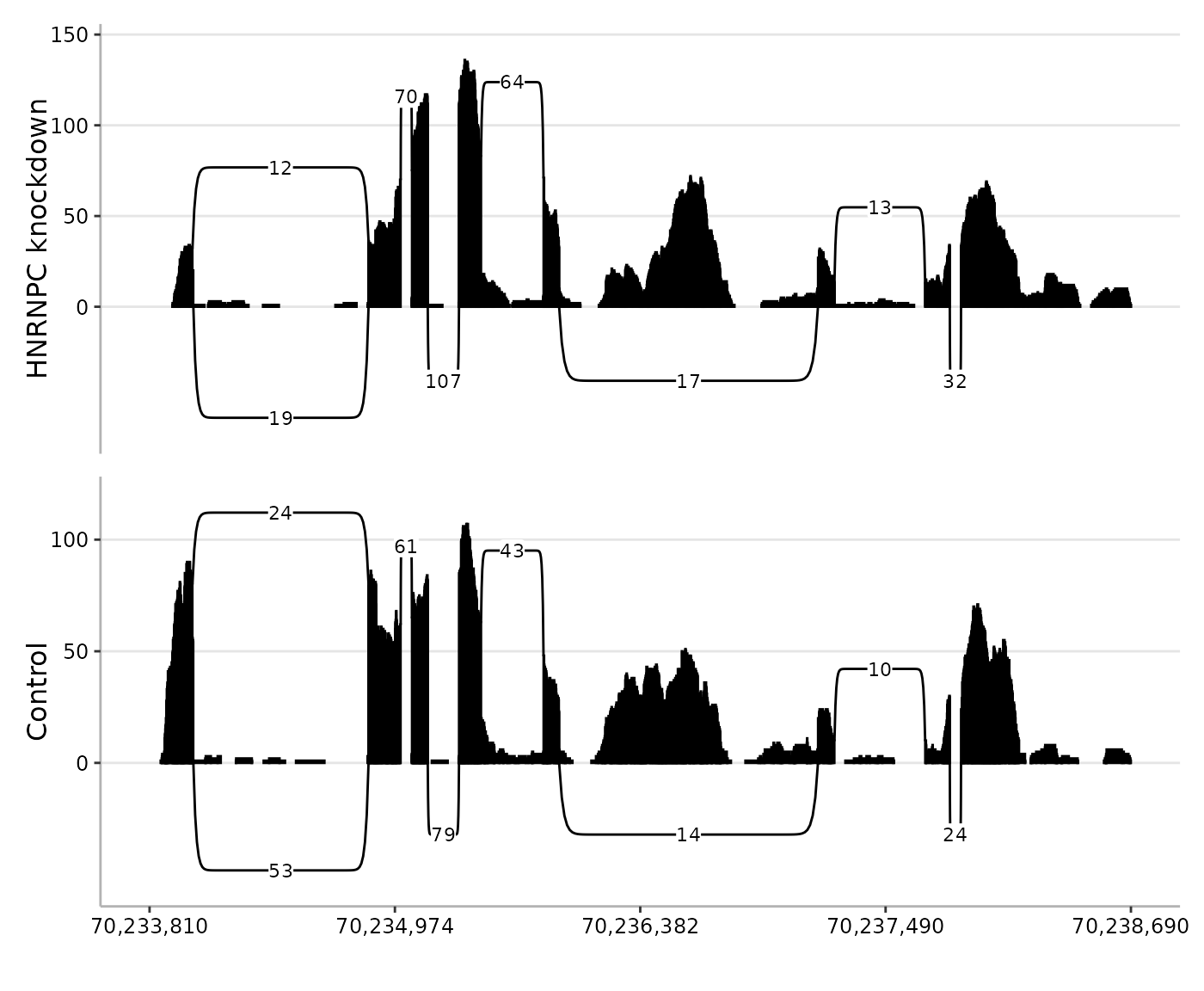
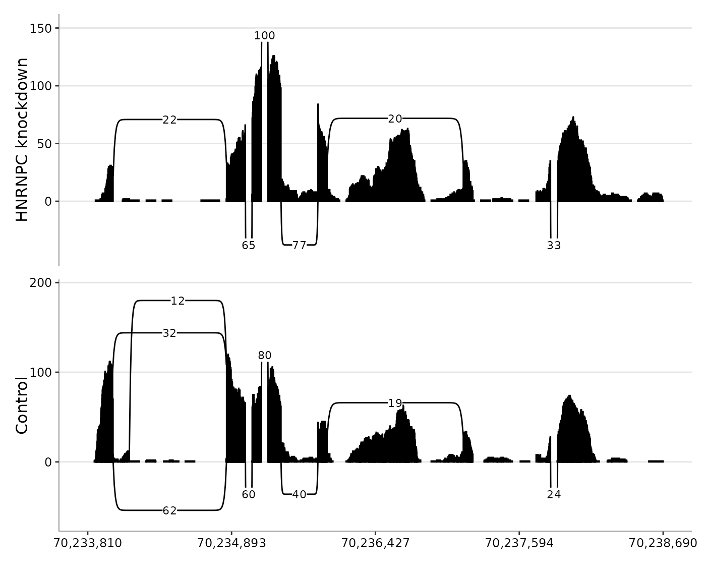
Specifying a stranded protocol for unstranded BAM files filters reads by strand. As a result, either "reverse" or "forward" shows only part of the coverage that is visible when strandedness = "unstranded".

spliceTerrain(
    bam = bams,
    region = region,
    strandedness = "forward"
)

spliceTerrain(
    bam = bams,
    region = region,
    strandedness = "reverse"
)

For paired-end BAM files, spliceTerrain() detects paired-end status from the BAM alignment flags and imports alignments accordingly. Mapped reads are retained even when their mates are unmapped. Read-one/read-two flags determine strand interpretation for both complete pairs and singletons. Unmapped, secondary, supplementary, and below-min_mapq alignments are excluded. If region specifies a strand and strandedness is not "unstranded", alignments are restricted to the resolved region strand.

Coverage and junction support are fragment-level summaries. Each imported mate group, mapped singleton, or single-end read is one fragment. Coverage uses the union of each fragment’s aligned blocks. Overlapping mates contribute at most one count per covered position. Introns and unsequenced gaps between mates remain uncovered. Each fragment supports a distinct junction at most once, even if both mates cross it.

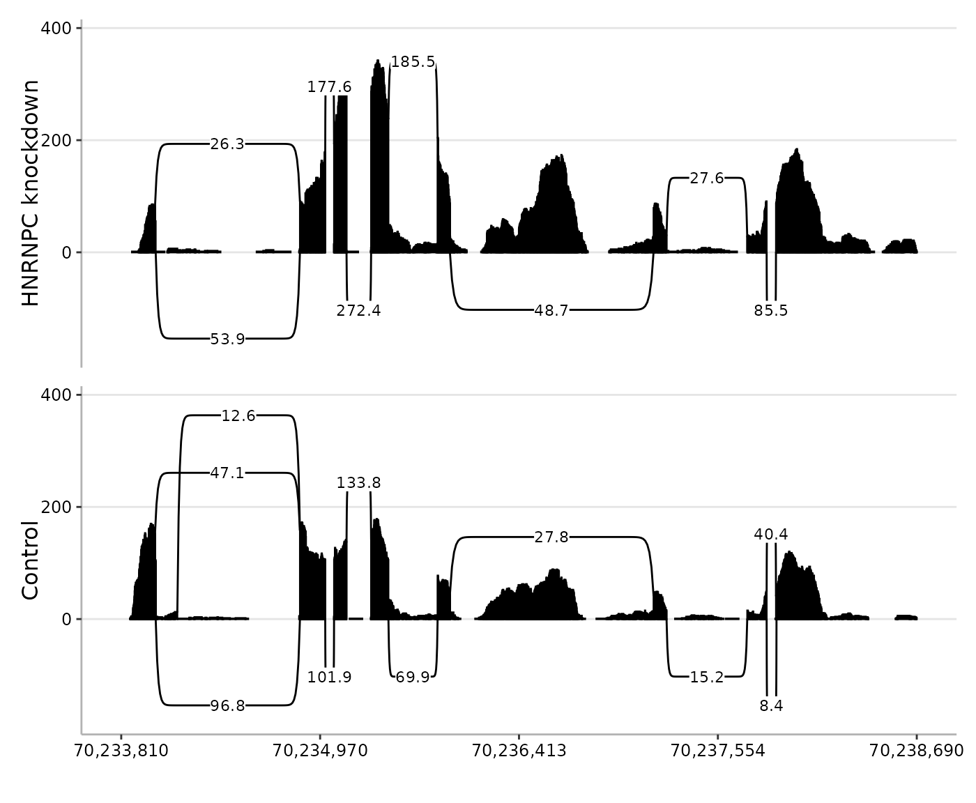
Normalising between samples

When samples have different sequencing depths, coverage and junction counts can be normalised with lib_size. Supply full-library sizes in fragment units before restriction to the plotting region: one per pair or mapped singleton, or one per read for single-end data. Additional normalisation factors, such as trimmed mean of M-values (TMM) factors (Robinson and Oshlack 2010) estimated with edgeR, can be supplied with norm_factors. The effective library size is calculated as lib_size * norm_factors.

By default, counts are normalised to the median effective library size. Use normalise_to to set the target explicitly. The common_y argument is useful when comparing samples because it puts sample panels on the same y-axis scale.

spliceTerrain(
    bam = bams,
    region = region,
    lib_size = c(40e6, 55e6),
    norm_factors = c(0.95, 1.08),
    normalise_to = 50e6,
    common_y = TRUE
)

Compressed genomic layouts

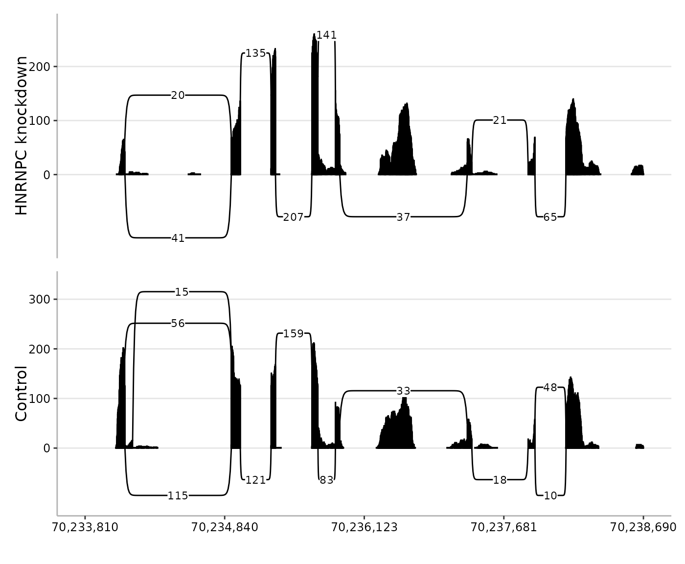
By default, compress_introns = TRUE compacts large uninformative gaps so the plot focuses on observed signal. The intron_width argument controls the approximate width of compacted introns in plot space. The map is built jointly from retained coverage across samples, annotations, and junction/selection anchors. Retained blocks keep their widths; gaps between them receive the chosen width. Consequently, retained intronic coverage or an unannotated covered exon remains part of the displayed signal rather than being compressed simply because it lies inside an annotated intron. Changing coverage filters can change the retained blocks and their map.

spliceTerrain(
    bam = bams,
    region = region,
    compress_introns = TRUE,
    intron_width = 500
)

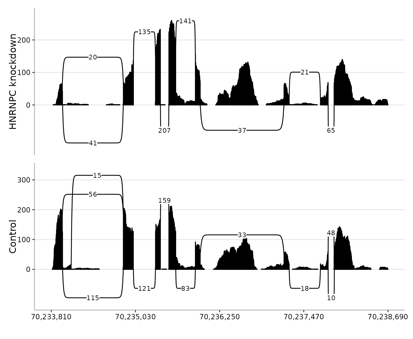
If exact genomic distances are more important than compact display, intron compression can be disabled.

spliceTerrain(
    bam = bams,
    region = region,
    compress_introns = FALSE
)

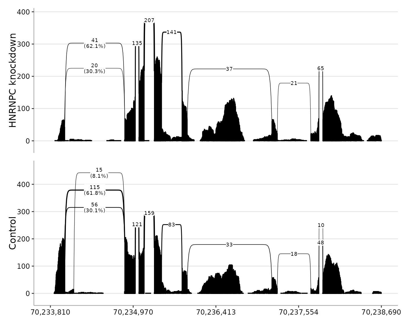
Junction arc display

Junction arcs can be tuned with arc_height, arc_side, and arc_scale. Increasing arc_height gives stacked arcs more vertical separation. The arc_side argument controls whether arcs are drawn above, below, or on both sides of the coverage track. With arc_scale = TRUE, arc width scales with filtered fragment support. Junction label size is controlled with junc_text_size.

spliceTerrain(
    bam = bams,
    region = region,
    junction_usage = "chr14:70234854-70234854",
    arc_height = 2,
    arc_side = "above",
    arc_scale = TRUE,
    junc_text_size = 2.5
)

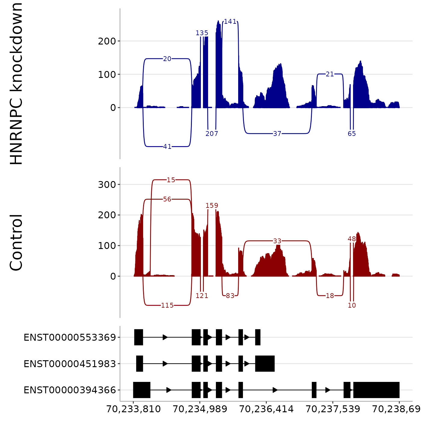
Sample colours and panel layout

The colours argument controls the colours used for sample coverage and junction arcs. It can be a single colour used for all samples or one colour per BAM file.

Axis text sizes can be adjusted with axis_title_size and axis_text_size.

spliceTerrain(
    bam = bams,
    region = region,
    annotation = annotation,
    colours = c("darkblue", "darkred"),
    panel_heights = c(2, 2, 1),
    axis_title_size = 20,
    axis_text_size = 12
)

Returning and reusing plot data

Most users can work directly with the final plot returned by spliceTerrain(). For advanced workflows, set return_ctx = TRUE to return the processed context instead. This contains validated settings, imported alignments, summarised coverage, junction counts, annotation, and overlays. The gal field contains one alignment object per sample: GAlignments for single-end BAMs or GAlignmentsList for paired-end BAMs. The paired-end list groups imported mates and includes mapped singleton reads. The cov and juncs fields contain fragment summaries: coverage_raw holds unnormalised fragment counts and coverage holds the plotting values after any library-size normalisation. The juncs_all field retains eligible junction summaries on the plotting chromosome before display filtering or clipping, including out-of-window junctions from imported alignments. It provides a stable reference for the usage_fraction column in juncs. That column is on the 0–1 scale, with NA for unselected junctions or an undefined percentage. All coordinate-bearing fields use genomic coordinates; compressed plot coordinates are generated internally only when the context is plotted.

The context also supports programmatic inspection, including AI-assisted workflows. Scripts or AI agents working within an R session can inspect coverage and junction summaries, check the values underlying plotted labels, and modify annotations or plotting settings before redrawing the figure. This provides access to the data behind the visualisation without requiring those values to be inferred from the plot image.

ctx <- spliceTerrain(
    bam = bams,
    region = region,
    annotation = annotation,
    min_junction_reads = 1,
    panel_heights = c(2, 2, 1),
    min_arrow = 100,
    return_ctx = TRUE
)

names(ctx)
#>  [1] "bam"                      "region"                   "annotation"               "junction_usage"           "junction_usage_label_sep" "highlight"                "strandedness"             "min_mapq"                 "min_coverage"             "min_junction_reads"       "lib_size"                 "norm_factors"             "normalise_to"             "compress_introns"         "intron_width"             "min_arrow"                "common_y"                 "arc_height"               "arc_side"                 "arc_scale"                "colours"                  "highlight_colour"         "anno_fill_by"             "anno_fill_colours"        "anno_label_by"            "anno_label_colour"        "anno_label_size"          "junc_text_size"           "panel_heights"            "axis_title_size"          "axis_text_size"           "annotated_junctions"      "gal"                      "cov"                      "juncs"                    "juncs_all"

The context can be passed back with the ctx argument to redraw the plot without re-importing BAM files or recalculating coverage and junctions. For example, the annotation can be used to retain only coverage overlapping annotated exons and junctions that exactly match annotated introns.

ctx$cov <- ctx$cov[overlapsAny(ctx$cov, ctx$annotation)]
ctx$juncs <- ctx$juncs[ctx$juncs$annotation_match]
spliceTerrain(ctx = ctx)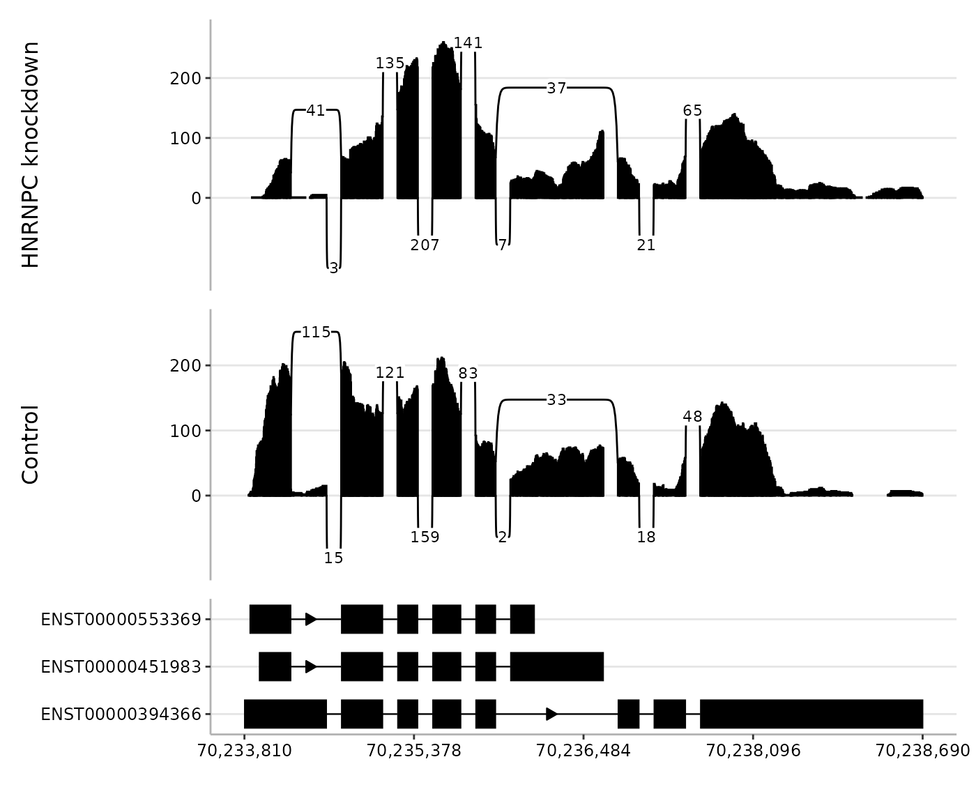

The annotation_match field records whether each junction exactly matches an intron implied by the supplied annotation. Plotting settings can also be changed directly, for example with ctx$colours <- c("darkblue", "darkred"). Settings that control BAM import, filtering, or normalisation are not reapplied when a context is replotted because its coverage and junctions are already processed.

Filtering ctx$juncs changes which arcs are displayed without changing the usage denominator. Changing ctx$junction_usage to another GRanges selection recalculates the fractions from ctx$juncs_all when plotting. If you intend to change the reference evidence itself, edit ctx$juncs_all, retaining one row per sample/junction.

Session information

sessionInfo() |>
    pander()

R Under development (unstable) (2026-11-03 r90835)

Platform: x86_64-pc-linux-gnu

locale: LC_CTYPE=C.UTF-8, LC_NUMERIC=C, LC_TIME=C.UTF-8, LC_COLLATE=C.UTF-8, LC_MONETARY=C.UTF-8, LC_MESSAGES=C.UTF-8, LC_PAPER=C.UTF-8, LC_NAME=C, LC_ADDRESS=C, LC_TELEPHONE=C, LC_MEASUREMENT=C.UTF-8 and LC_IDENTIFICATION=C

attached base packages: stats4, stats, graphics, grDevices, utils, datasets, methods and base

other attached packages: GenomeInfoDb(v.1.48.0), pander(v.0.6.6), scales(v.1.4.0), EnsDb.Hsapiens.v75(v.2.99.0), ensembldb(v.2.36.1), AnnotationFilter(v.1.36.0), GenomicFeatures(v.1.64.0), AnnotationDbi(v.1.74.0), Biobase(v.2.72.0), GenomicRanges(v.1.64.0), Seqinfo(v.1.2.0), IRanges(v.2.46.0), S4Vectors(v.0.50.3), BiocGenerics(v.0.58.1), generics(v.0.1.4), RNAseqData.HNRNPC.bam.chr14(v.0.50.0), spliceTerrain(v.0.99.0) and BiocStyle(v.2.40.0)

loaded via a namespace (and not attached): farver(v.2.1.2), blob(v.1.3.0), Biostrings(v.2.80.2), S7(v.0.2.2), bitops(v.1.1-0), fastmap(v.1.2.0), RCurl(v.1.98-1.20), lazyeval(v.0.2.3), GenomicAlignments(v.1.48.0), XML(v.3.99-0.25), digest(v.0.6.39), lifecycle(v.1.0.5), ProtGenerics(v.1.44.0), KEGGREST(v.1.52.2), RSQLite(v.3.53.3), compiler(v.4.7.0), rlang(v.1.3.0), sass(v.0.4.10), tools(v.4.7.0), yaml(v.2.3.12), rtracklayer(v.1.72.0), knitr(v.1.52), labeling(v.0.4.3), S4Arrays(v.1.12.1), bit(v.4.6.0), curl(v.8.1.0), DelayedArray(v.0.38.2), RColorBrewer(v.1.1-3), abind(v.1.4-8), BiocParallel(v.1.46.0), withr(v.3.0.3), desc(v.1.4.3), grid(v.4.7.0), ggplot2(v.4.0.3), SummarizedExperiment(v.1.42.0), cli(v.3.6.6), rmarkdown(v.2.32), crayon(v.1.5.3), ragg(v.1.5.2), otel(v.0.2.0), httr(v.1.4.9), rjson(v.0.2.23), DBI(v.1.3.0), cachem(v.1.1.0), parallel(v.4.7.0), BiocManager(v.1.30.27), XVector(v.0.52.0), restfulr(v.0.0.17), matrixStats(v.1.5.0), vctrs(v.0.7.3), Matrix(v.1.7-6), jsonlite(v.2.0.0), bookdown(v.0.48), patchwork(v.1.3.2), bit64(v.4.8.6), systemfonts(v.1.3.2), jquerylib(v.0.1.4), glue(v.1.8.1), pkgdown(v.2.2.1), codetools(v.0.2-20), gtable(v.0.3.6), BiocIO(v.1.22.0), UCSC.utils(v.1.8.0), htmltools(v.0.5.9), R6(v.2.6.1), textshaping(v.1.0.5), evaluate(v.1.0.5), lattice(v.0.23-1), png(v.0.1-9), Rsamtools(v.2.28.0), cigarillo(v.1.2.1), memoise(v.2.0.1), bslib(v.0.12.0), Rcpp(v.1.1.2), SparseArray(v.1.12.3), xfun(v.0.62), pkgconfig(v.2.0.3), fs(v.2.1.0) and MatrixGenerics(v.1.24.0)

References

Garrido-Martín, Diego, Emilio Palumbo, Roderic Guigó, and Alessandra Breschi. 2018. “ggsashimi: Sashimi Plot Revised for Browser- and Annotation-Independent Splicing Visualization.” PLOS Computational Biology 14 (8): e1006360. https://doi.org/10.1371/journal.pcbi.1006360.

Hahne, Florian, and Robert Ivanek. 2016. “Visualizing Genomic Data Using Gviz and Bioconductor.” In Statistical Genomics: Methods and Protocols, edited by Ewy Mathé and Sean Davis. Springer New York. https://doi.org/10.1007/978-1-4939-3578-9_16.

Katz, Yarden, Eric T. Wang, Jacob Silterra, et al. 2015. “Quantitative Visualization of Alternative Exon Expression from RNA-seq Data.” Bioinformatics 31 (14): 2400–2402. https://doi.org/10.1093/bioinformatics/btv034.

Lawrence, Michael, Wolfgang Huber, Hervé Pagès, et al. 2013. “Software for Computing and Annotating Genomic Ranges.” PLOS Computational Biology 9 (8): e1003118. https://doi.org/10.1371/journal.pcbi.1003118.

Robinson, Mark D., and Alicia Oshlack. 2010. “A Scaling Normalization Method for Differential Expression Analysis of RNA-seq Data.” Genome Biology 11 (3): R25. https://doi.org/10.1186/gb-2010-11-3-r25.

Wong, Alex C. H., Justin J.-L. Wong, John E. J. Rasko, and Ulf Schmitz. 2024. “SpliceWiz: Interactive Analysis and Visualization of Alternative Splicing in R.” Briefings in Bioinformatics 25 (1): bbad468. https://doi.org/10.1093/bib/bbad468.

Yin, Tengfei, Dianne Cook, and Michael Lawrence. 2012. “ggbio: An R Package for Extending the Grammar of Graphics for Genomic Data.” Genome Biology 13 (8): R77. https://doi.org/10.1186/gb-2012-13-8-r77.

Zarnack, Kathi, Julian König, Mojca Tajnik, et al. 2013. “Direct Competition Between hnRNP C and U2AF65 Protects the Transcriptome from the Exonization of Alu Elements.” Cell 152 (3): 453–66. https://doi.org/10.1016/j.cell.2012.12.023.

Lachlan Baer

Last modified: 2026-11-05

Installation and setup

Quick start

Introduction

Motivation

Complete guide

Input BAM files and regions

Adding transcript annotation

Styling annotation tracks

Highlighting regions of interest

Local junction-usage labels

Why this is not event-level PSI

Filtering signal

Stranded RNA-seq data

Normalising between samples

Compressed genomic layouts

Junction arc display

Sample colours and panel layout

Returning and reusing plot data

Session information

References

Creating Sashimi-Style Plots with `spliceTerrain`

Lachlan Baer

Last modified: 2026-11-05

Installation and setup

Quick start

Introduction

Motivation

Related tools

Complete guide

Input BAM files and regions

Adding transcript annotation

Styling annotation tracks

Highlighting regions of interest

Local junction-usage labels

Why this is not event-level PSI

Filtering signal

Stranded RNA-seq data

Normalising between samples

Compressed genomic layouts

Junction arc display

Sample colours and panel layout

Returning and reusing plot data

Session information

References